Centered Kernel Alignment (CKA) in Detail
CKA is a state-of-the-art tool to measure the similarity of neural network representations, but in this post, I walk through its derivation in detail for a deeper understanding. [Original paper]
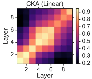 CKA map example from original paper
1. Overview
CKA (Centered Kernel Alignment) is a state-of-the-art tool for measuring the similarity of neural network representations. It has practical uses such as comparing layers within a single model, comparing representations across two different architectures, or studying how representations evolve during training. After reading the original paper, I wanted more intuition about how the CKA formulae capture similarity, so I spent some time breaking it down. This post is a summary of my understanding of CKA and the derivations I worked out.
In summary, the key insight of CKA is the use of gram matrices that collapse the neuron dimension and instead compare inter-sample similarities, making the measure invariant to the width or bases of the layers being compared.
2. Inputs and Outputs
To run CKA, we must have 2 matrices of paired activations (aka representations) from the same neural network, or different neural networks.
Let’s call these matrices $X$ and $Y$. Let $X \in \mathbb{R}^{n \times d_1}$ and $Y \in \mathbb{R}^{n \times d_2}$, where $n$ is the number of samples and $d_i$ is the dimensionality of the representations. $d_1$ and $d_2$ can be different, but $n$ must be the same for both matrices as these represent paired samples. This means CKA lets us compare the similarity of representations that come from layers of differing widths. We also assume that these matrices have been centered, that is, the column means have been subtracted. Centering ensures the similarity measure is not skewed by constant offsets in activations, and is required for the HSIC connection discussed in Section 3.
3. Formula
One formula for (linear) CKA is given by: $$\text{CKA}(X,Y) = \frac{\lVert Y^TX \rVert_F^2}{\lVert X^TX \rVert_F \lVert Y^TY \rVert_F}$$
Let’s break down this equation:
-
Breaking down the Numerator
Let’s first look at the numerator of the formula: $$\lVert Y^TX \rVert_F^2$$ In Section 3 of Similarity of Neural Network Representations Revisited, we are shown a way to link from dot products between examples to dot products between features: $$ \lVert Y^TX \rVert_F^2 = \langle \text{vec}(XX^T), \text{vec}(YY^T)\rangle$$ This is the key insight of CKA, where a computation comparing the multivariate features between the two matrices can actually translate to computing the similarity between examples, and then comparing the resulting similarity structures. We will expand the formulation as follows in order to reach the intuition presented by the authors.
We will work this the opposite way here, including more details to understand the intermediate steps. First, we will establish an important property of the Frobenius norm, and of the trace.-
frobenius norm reformulation: $\lVert A \rVert_F = \sqrt{\text{Tr}(A^TA)}$
-
trace property (cyclic property): $\text{Tr}(ABC) = \text{Tr}(CAB) = \text{Tr}(BCA)$
Now, we can rewrite the numerator of the CKA formula as follows:
-
- Connection to the Hilbert Schmidt Independence Criterion
Before formulating the connection to the Hilbert-Schmidt Independence Criterion (HSIC), we’ll first recall the definition of the cross-covariance matrix $$\text{cov}(X,Y) = \frac{1}{n-1}\left(X - \mathbb{E}(X)\right)\left(Y - \mathbb{E}(Y)\right)^T$$ Now, we will connect the trace formulation from above to the covariance matrix. Remember that we assume our data matrices are already centered
However, HSIC is not invariant to isotropic scaling — i.e., it does not satisfy $s(X,Y) = s(\alpha X, \beta Y)$ for a similarity index $s$. For CKA, we would like this property so that the score is not affected by the scale of the activations. Therefore, the authors propose a normalized version. We now derive the simplifications for both the linear kernel and the arbitrary kernel cases. For the linear kernel, we have: $$ \text{HSIC}(X,Y) = \frac{1}{(n-1)^2}\text{Tr}(X^TXY^TY) $$
For linear CKA, we get:
For an arbitrary kernel $K, L$, we simplify CKA as follows:
Together, these two formulations give a practical and kernel-flexible way to compare neural network representations, invariant to isotropic scaling and applicable across layers of any width.
Neha Verma
PhD Student
I am a PhD student at Johns Hopkins Center for Language and Speech Processing.